Causal Inference with Bayesian Networks. Main Concepts and Methods
1. Causality
1.1 Why is causality important?
Experts and practitioners in various domains are commonly interested in discovering causal relationships to answer questions like
“What drives economical prosperity?”, “What fraction of patients can a given drug save?”, “How much would a power failure cost to a given manufacturing plant?”.
The ability to identify truly causal relationships is fundamental to developing impactful interventions in medicine, policy, business, and other domains.
Often, in the absence of randomised control trials, there is a need for causal inference purely from observational data. However, in this case the commonly known fact that
correlation does not imply causation
comes to life. Therefore, it is crucial to distinguish between events that cause specific outcomes and those that merely correlate. One possible explanation for correlation between variables where neither causes the other is the presence of confounding variables that influence both the target and a driver of that target. Unobserved confounding variables are severe threats when doing causal inference on observational data. The research community has made significant contributions to develop methods and techniques for this type of analysis. Potential outcomes framework (Rubin causal model), propensity score matching and structural causal models are, arguably, the most popular frameworks for observational causal inference.
Here, we focus on the structural causal models and one particular type, Bayesian Networks.
Interested users can find more details in the references below.
Lecture notes on potential outcomes approach, Dept of Psychiatry & Behavioral Sciences, Stanford University by Booil Jo;
Probabilistic graphical models: principles and techniques by D. Koller and N. Friedman.
1.2 Structural Causal Models (SCMs)
Structural causal models represent causal dependencies using graphical models that provide an intuitive visualisation by representing variables as nodes and relationships between variables as edges in a graph.
SCMs serve as a comprehensive framework unifying graphical models, structural equations, and counterfactual and interventional logic.
Graphical models serve as a language for structuring and visualising knowledge about the world and can incorporate both data-driven and human inputs.
Counterfactuals enable the articulation of something there is a desire to know, and structural equations serve to tie the two together.
SCMs had a transformative impact on multiple data-intensive disciplines (e.g. epidemiology, economics, etc.), enabling the codification of the existing knowledge in diagrammatic and algebraic forms and consequently leveraging data to estimate the answers to interventional and counterfacutal questions.
Bayesian Networks are one of the most widely used SCMs and are at the core of this library.
More on SCMs: Causality: Models, Reasoning, and Inference by J. Pearl.
2. Bayesian Networks (BNs)
2.1 Directed Acyclic Graph (DAG)
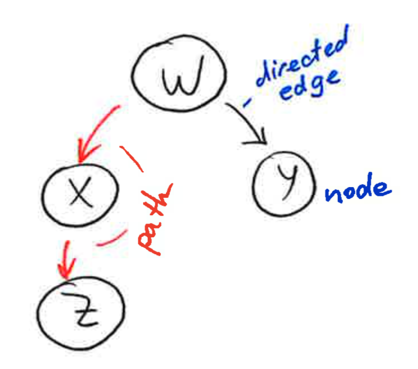
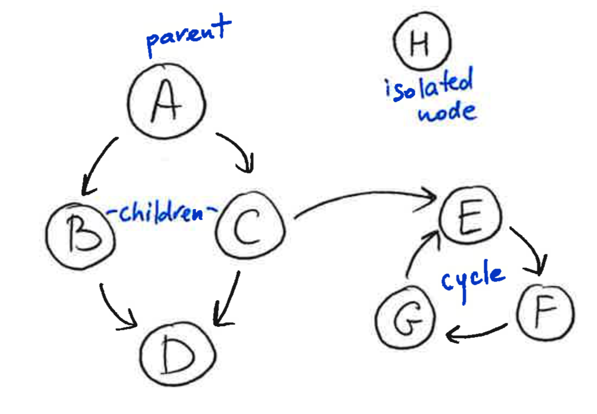
A graph is a collection of nodes and edges, where the nodes are some objects, and edges between them represent some connection between these objects. A directed graph, is a graph in which each edge is orientated from one node to another node. In a directed graph, an edge goes from a parent node to a child node. A path in a directed graph is a sequence of edges such that the ending node of each edge is the starting node of the next edge in the sequence. A cycle is a path in which the starting node of its first edge equals the ending node of its last edge. A directed acyclic graph is a directed graph that has no cycles.
2.2 What Bayesian Networks are and are not
What are Bayesian Networks?
Bayesian Networks are probabilistic graphical models that represent the dependency structure of a set of variables and their joint distribution efficiently in a factorised way.
Bayesian Network consists of a DAG, a causal graph where nodes represents random variables and edges represent the the relationship between them, and a conditional probability distribution (CPDs) associated with each of the random variables.
If a random variable has parents in the BN then the CPD represents \(P(\text{variable|parents}) \) i.e. the probability of that variable given its parents. In the case, when the random variable has no parents it simply represents \(P(\text{variable}) \) i.e. the probability of that variable.
Even though we are interested in the joint distribution of the variables in the graph, Bayes’ rule requires us to only specify the conditional distributions of each variable given its parents.
The links between variables in Bayesian Networks encode dependency but not necessarily causality. In this package we are mostly interested in the case where Bayesian Networks are causal. Hence, the edge between nodes should be seen as a cause -> effect relationship.
Let’s consider an example of a simple Bayesian network shown in figure below. It shows how the actions of customer relationship managers (emails sent and meetings held) affect the bank’s income.
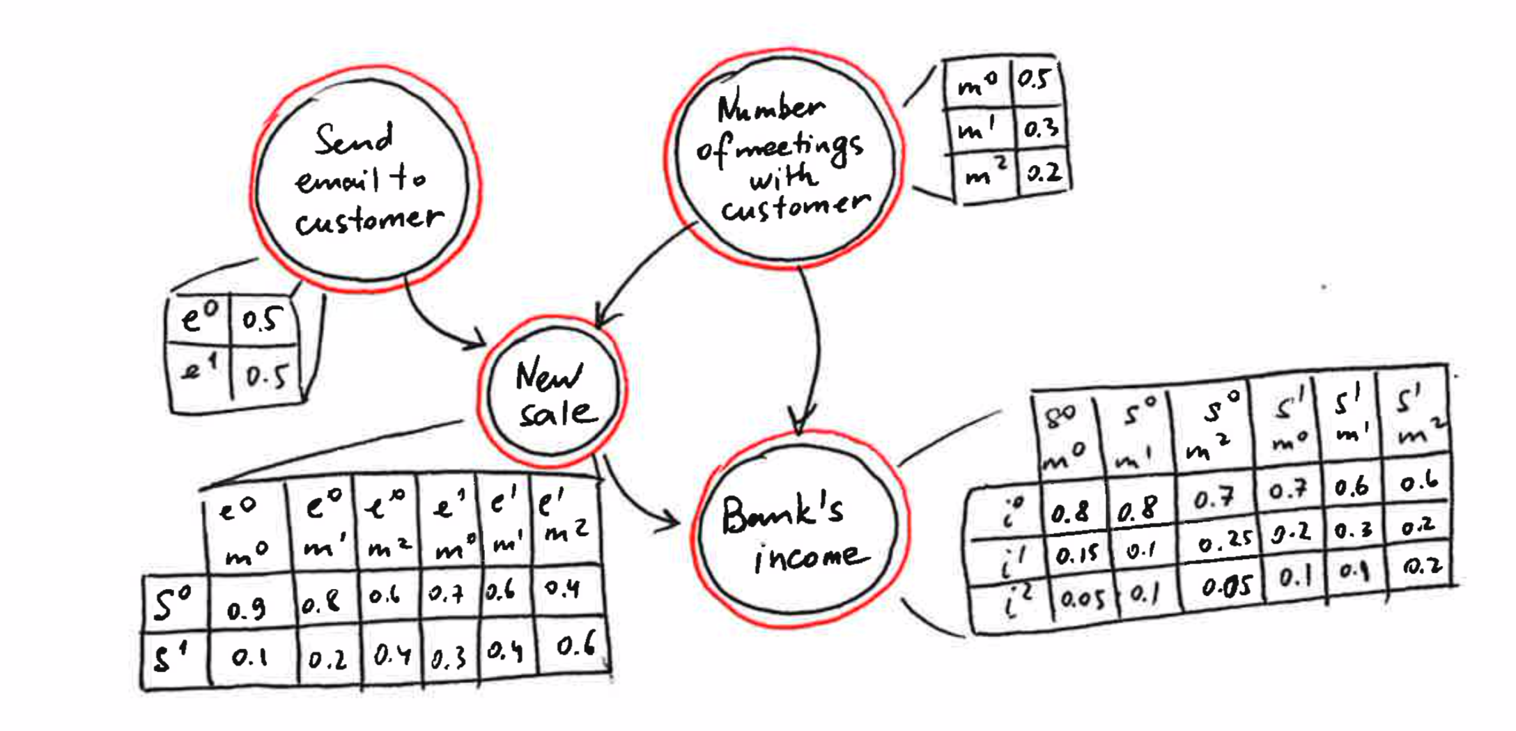
New sales and the number of meetings with a customer directly affect the bank’s income. However, these two drivers are not independent but the number of meetings also influences whether a new sale takes place. In addition, system prompts indirectly influence the bank’s income through the generation of new sales. This example shows that BNs are able to capture complex relationships between variables, represent dependencies between drivers, and include drivers that do not affect the target directly.
Steps for working with a Bayesian Network
BN models are built in a multi-step process before they can be used for analysis.
Structure Learning. The structure of a network describing the relationships between variables can be learned from data, or built from expert knowledge.
Structure Review. Each relationship should be validated, so that it can be asserted to be causal. This may involve flipping / removing / adding learned edges, or confirming expert knowledge from trusted literature or empirical beliefs.
Likelihood Estimation. The conditional probability distribution of each variable given its parents can be learned from data.
Prediction & Inference. The given structure and likelihoods can be used to make predictions, or perform observational and counterfactual inference. CausalNex supports structure learning from continuous data, and expert opinion. CausalNex supports likelihood estimation and prediction/inference from discrete data. A
Discretiserclass is provided to help discretising continuous data in a meaningful way.
Since BNs themselves are not inherently causal models, the structure learning algorithms on their own merely learn that there are dependencies between variables. A useful approach to the problem is to first group the features into themes and constrain the search space to inspect how themes of variables relate. If there is further domain knowledge available, it can be used as additional constraints before learning a graph algorithmically.
What can we use Bayesian Networks for?
The probabilities of variables in Bayesian Networks update as observations are added to the model. This is useful for inference or counterfactuals, and for predictive analytics. Metrics can help us understand the strength of relationships between variables.
The sensitivity of nodes to changes in observations of other events can be used to assess what changes could lead to what effects;
The active trail of a target node identifies which other variables have any effect on the target.
2.3 Advantages and Drawbacks of Bayesian Networks
Advantages
Bayesian Networks offer a graphical representation that is reasonably interpretable and easily explainable;
Relationships captured between variables in a Bayesian Network are more complex yet hopefully more informative than a conventional model;
Models can reflect both statistically significant information (learned from the data) and domain expertise simultaneously;
Multiple metrics can used to measure the significance of relationships and help identify the effect of specific actions;
Offer a mechanism of suggesting counterfactual actions and combine actions without aggressive independence assumptions.
Drawbacks
Granularity of modelling may have to be lower. However, this may either not be necessary, or can be run in tangent to other techniques that provide accuracy but are less interpretable;
Computational complexity is higher. However, this can be offset with careful feature selection and a less granular discretisation policy, but at the expense of predictive power;
This is (unfortunately) not a way of fully automating Causal Inference.
3. The BayesianNetwork Class
The BayesianNetwork class is the central class for the causal inference analysis in the package.
It is built on top of the StructureModel class, which is an extension of networkx.DiGraph
StructureModel represents a causal graph, a DAG of the respective BN and holds directed edges, describing
a cause -> effect relationship. In order to define the BayesianNetwork, users should provide a relevant StructureModel.
Cycles are permitted within a
StructureModelobject. However, only acyclic connectedStructureModelobjects are allowed in the construction ofBayesianNetwork; isolated nodes are not allowed.
3.1 Defining the DAG with StructureModel
Our package enables a hybrid way to learn structure of the model.
For instance, users can define a causal model fully manually, e.g., using the domain expertise:
    from causalnex.structure import StructureModel
    # Encoding the causal graph suggested by an expert
    #        d
    #     ↙  ↓  ↘
    #    a ← b → c
    #        ↑  ↗
    #        e
    sm_manual = StructureModel()
    sm_manual.add_edges_from(
        [
            ("b", "a"),
            ("b", "c"),
            ("d", "a"),
            ("d", "c"),
            ("d", "b"),
            ("e", "c"),
            ("e", "b"),
        ],
        origin="expert",
    )
Or, users can learn the network structure automatically from the data using the NOTEARS algorithm. Moreover, if there is domain knowledge available,
it can be used as additional constraints before learning a graph algorithmically.
NOTEARS is a recently published algorithm for learning DAGs from data, framed as a continuous optimisation problem. It allowed us to overcome the challenges of combinatorial optimisation, giving a new impetus to the usage of BNs in machine learning applications.
    from causalnex.structure.notears import from_pandas
    from causalnex.network import BayesianNetwork

    # Unconstrained learning of the structure from data
    sm = from_pandas(data)
    # Imposing edges that are not allowed in the causal model
    sm_with_tabu_edges = from_pandas(data, tabu_edges=[("e", "a")])
    # Imposing parent nodes that are not allowed in the causal model
    sm_with_tabu_parents = from_pandas(data, tabu_parent_nodes=["a", "c"])
    # Imposing child nodes that are not allowed in the causal model
    sm_with_tabu_parents = from_pandas(data, tabu_child_nodes=["d", "e"])
Finally, the output of the algorithm should be inspected, and adjusted if required, by a domain expert. This is a targeted effort to encode important domain knowledge in models, and avoid spurious relationships.
    # Removing the learned edge from the model
    sm.remove_edge("a", "c")
    # Changing the direction of the learned edge
    sm.remove_edge("c", "d")
    sm.add_edge("d", "c", origin="learned")
    # Adding the edge that was not learned by the algorithm
    sm.add_edge("a", "e", origin="expert")
When defining the structure model, we recommend using the entire dataset without discretisation of continuous variables.
3.2 Likelihood Estimation and Predictions with BayesianNetwork
Once the graph has been determined, the BayesianNetwork can be initialised and the conditional probability distributions of the variables can be learned from the data.
Maximum likelihood or Bayesian parameter estimation can be used for learning the CPDs.
When learning CPDs of the BN,
The dicscretised data should be used (either high or low granularity of features and target variables can be used);
Overfitting and underfitting of CPDs can be avoided with an appropriate train/test split of the data.
    from causalnex.network import BayesianNetwork
    from causalnex.discretiser import Discretiser

    # Inititalise BN with defined structure model
    bn = BayesianNetwork(sm)
    # First, learn all the possible states of the nodes using the whole dataset
    bn.fit_node_states(data_discrete)
    # Fit CPDs using the training dataset with the discretised continuous variable "c"
    train_data_discrete = train_data.copy()
    train_data_discrete["c"] = Discretiser(method="uniform").transform(discretised_data["c"].values)
    bn.fit_cpds(train_data_discrete, method="BayesianEstimator", bayes_prior="K2")
Once the CPDs are learned, they can be used to predict the state of a node as well as probability of each possible state of a node, based on some input data (e.g., previously unseen test data) and learned CPDs:
    predictions = bn.predict(test_data_discrete, "c")
    predicted_probabilities = bn.predict_probability(test_data_discrete, "c")
When all parents of a given node exist within input data, the method inspects the CPDs directly and avoids traversing the full network. When some parents do not exist within input data, the most likely state for every node that is not contained within data is computed, and the predictions are made accordingly.
4. Querying model and making interventions with InferenceEngine
After iterating over the model structure, CPDs, and validating the model quality, we can undertake inference on a BN to examine expected behaviour and gain insights.
InferenceEngine class provides methods to query marginals based on observations and to make interventions (a.k.a. DO-calculus) on a Bayesian Network.
4.1 Querying marginals with InferenceEngine.query
Inference and observation of evidence are done on the fly, following a deterministic Junction Tree Algorithm (JTA).
To query the model for baseline marginals that reflect the population as a whole, a query method can be used.
We recommend to update the model using the complete dataset for this type of queries.
    from causalnex.inference import InferenceEngine

    # Updating the model on the whole dataset
    bn.fit_cpds(data_discrete, method="BayesianEstimator", bayes_prior="K2")
    ie = InferenceEngine(bn)
    # Querying all the marginal probabilities of the model's distribution
    marginals = ie.query({})
Users can also query the marginals of states in a BN given some observations. These observations can be made anywhere in the network; the marginal distributions of nodes (including the target variable) will be updated and their impact will be propagated through to the node of interest:
    # Querying the marginal probabilities of the model's distribution
    # after an observed state of the node "b"
    marginals_after_observations = ie.query({"b": True})
For complex networks, the JTA may take an hour to update the probabilities throughout the network;
This process can not be parallelised, but multiple queries can be run in parallel;
4.2 Making interventions (Do-calculus) with InferenceEngine.do_intervention
Finally, users can use the insights from the inference and observation of evidence to encode taking actions and observe the effect of these actions on the target variable.
Our package supports simple Do-Calculus, allowing as to Make an intervention on the Bayesian Network.
Users can apply an intervention to any node in the data, updating its distribution using a do operator, examining the effect of that intervention by querying marginals and resetting any interventions:
    # Doing an intervention to the node "d"
    ie.do_intervention("d", True)
    # Querying all the updated marginal probabilities of the model's distribution
    marginals_after_interventions = ie.query({})
    # Re-introducing the original conditional dependencies
    ie.reset_do("d")